Indexed operations for non-rectangular lattices applied to convolutional neural networks
This section presents the content of the paper
Jacquemont, M.; Antiga, L.; Vuillaume, T.; Silvestri, G.; Benoit, A.; Lambert, P. and Maurin, G. (2019). Indexed Operations for Non-rectangular Lattices Applied to Convolutional Neural Networks. In Proceedings of the 14th International Joint Conference on Computer Vision, Imaging and Computer Graphics Theory and Applications - Volume 5: VISAPP, ISBN 978-989-758-354-4, pages 362-371. DOI: 10.5220/0007364303620371, https://hal.science/hal-02087157/
The content of this section, as well as the associated images, are distributed under a CC BY-NC-ND 4.0 DEED license. You can find more information about this license here: https://creativecommons.org/licenses/by-nc-nd/4.0/
Mikael Jacquemont1,2, Luca Antiga3, Thomas Vuillaume1, Giorgia Silvestri3, Alexandre Benoit2, Patrick Lambert2 and Gilles Maurin1
1 Laboratoire d’Annecy de Physique des Particules, CNRS, Univ. Savoie Mont-Blanc, Annecy, France, firstname.name@lapp.in2p3.fr
2 LISTIC, Univ. Savoie Mont-Blanc, Annecy, France, firstname.name@univ-smb.fr
3 Orobix, Bergamo, Italy, firstname.name@orobix.com
INTRODUCTION
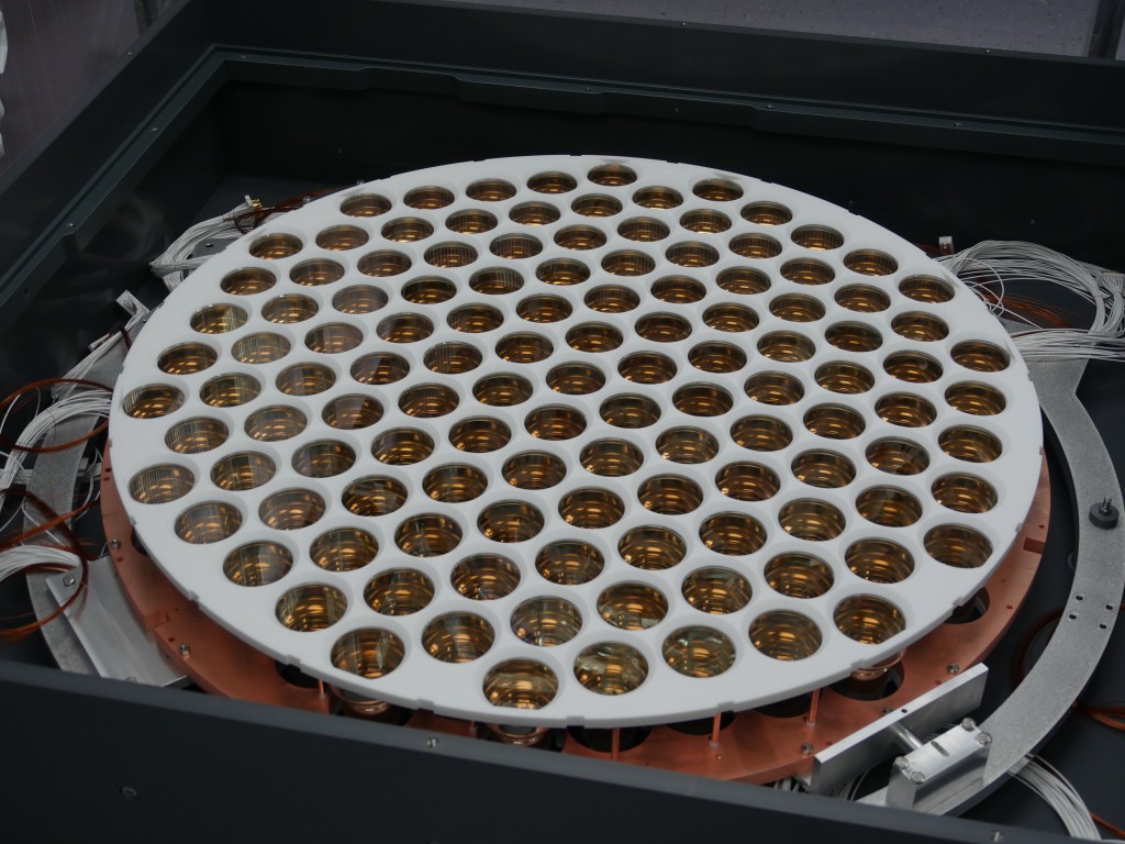
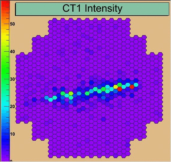
Traditional convolutional kernels have been developed for rectangular and regular pixel grids as found in traditional images. However, some imaging sensors present different shapes and do not have regularly spaced nor rectangular pixel lattices. This is particularly the case in science experiments where sensors use various technologies and must answer specific technological needs. Examples (displayed in figure 1) of such sensors in physics include the XENON1T experiment [Scovell13], the KM3NeT experiment [Kat12] or Imaging Atmospheric Cherenkov Telescope (IACT) cameras such as the ones of H.E.S.S. [BCG+14] or the Cherenkov Telescope Array (CTA) (NectarCam, [GlicensteinBarceloBarrio+13]; LSTCam, [AAB+13]; and FlashCam, [PuhlhoferBauerBiland+12]).
A traditional approach to overcome this and use traditional convolution neural network framework out of the box is to over-sample the image into a Cartesian grid. For regular lattices, such as hexagonal ones, it is also possible to apply geometrical transformation to the images to shift them into Cartesian grids. In that case, masked convolutions can be used to respect the original layout of the images, like in HexaConv [HPCW18]. In this paper, the authors present group convolutions for square pixels and hexagonal pixel images. A group convolution consists in applying several transformations (e.g. rotation) to the convolution kernel to benefit from the axis of symmetry of the images. In the hexagonal grid case they use masked convolutions applied to hexagonal pixel images represented in the Cartesian grid (via shifting).
However, such approaches may have several drawbacks:
oversampling or geometric transformation may introduce distortions that can potentially result in lower accuracy or unexpected results;
oversampling or geometric transformation impose additional processing, often performed at the CPU level which slows inference in production;
geometric transformation with masked convolution adds unnecessary computations as the mask has to be applied to the convolution kernel at each iteration;
oversampling or geometric transformations can change the image shape and size.
In order to prevent these issues and be able to work on unaltered data, we present here a way to apply convolution and pooling operators to any grid, given that each pixel neighbor is known and provided. This solution, denoted indexed operations in the following, driven by scientific applications, is applied to an hexagonal kernel since this is one of the most common lattice besides the Cartesian one. However, indexed convolution and pooling are very general solutions, easily applicable to other domains with irregular grids.
At first, a reminder of how convolution and pooling work and are usually implemented is done. Then we present our custom indexed kernels for convolution and pooling. This solution is then applied to standard datasets, namely CIFAR-10 and AID to validate the approach and test performances. Finally, we discuss the results obtained as well as potential applications to real scientific use cases.
CONVOLUTION
Background
Convolution is a linear operation performed on data over which neighborhood relationships between elements can be defined. The output of a convolution operation is computed as a weighted sum (i.e. a dot product) over input neighborhoods, where the weights are reused over the whole input. The set of weights is referred to as the convolution kernel. Any input data can be vectorized and then a general definition of convolution can be defined as:
where \(K\) is the number of elements in the kernel, \(w_k\) is the value of the \(k\)-th weight in the kernel, and \(N_{jk}\) is the index of the \(k\)-th neighbor of the \(j\)-th neighborhood.
This general formulation of discrete convolution can be then made more specific for data over which neighborhood relationships are inherent in the structure of the input, such as 1D (temporal), 2D (image) and 3D (volumetric) data. For instance, in the case of classical images with square pixels, we define convolution as:
where the convolution kernel is a square matrix of size \((2W+1, 2H+1)\) and neighborhoods are implicitly defined through corresponding relative locations from the center pixel. Analogous expressions can be defined in N dimensions.
Since the kernel is constant over the input, i.e. its values do not depend on the location over the input, convolution is a linear operation. In addition, it has the advantage of accounting for locality and translation invariance, i.e. output values solely depend on input values in local neighborhoods, irrespective of where in the input those values occur.
Convolution cannot be performed when part of the neighborhood cannot be defined, such as at the border of an image. In this case, either the corresponding value in the output is skipped, or neighborhoods are extended beyond the reach of the input, which is referred to as padding. Input values in the padded region can be set to zero, or reproduce the same values as the closest neighbors in the input.
It is worth noting that the convolution can be computed over a subset of the input elements. On regular lattices this results in choosing one every \(n\) elements in each direction, an amount generally referred as stride. The larger the stride, the smaller the size of the output.
The location of neighbors in convolution kernels does not need to be adjacent, as it is in the image formulation above. Following the first expression, neighborhoods can be defined arbitrarily, in terms of shape and location of the neighbors. In case of regular lattices the amount of separation between the elements of a convolution kernel in each direction is referred to as dilation or atrous convolution [HKMMT90]. The larger the dilation, the further away from the center the kernel reaches out in the neighborhood.
In case of inputs with multiple channels such as an RGB images, or multiple features in intermediate layers in a neural network, all input channels contribute to the output and convolution is simply obtained as the sum of dot products over all the individual channels to produce output values. Equation (1) shows the 2D image convolution case with \(C\) input channels.
Therefore, the size of kernels along the channel direction determines the number of input features that the convolution operation expects, while the number of individual kernels employed in a neural network layer determines the number of features in the output.
Implementation
In neural network applications convolutions are performed over small spatial neighborhoods (e.g. \(3 \times 3\), \(5 \times 5\) for 2D images). Given the small size of the elements in the dot product, the most computationally efficient strategy for computing the convolution is not an explicitly nested loop as described on equation (1), but a vectorized dot product over all neighborhoods. Then, as most deep learning frameworks intensively do, one can make use of the highly optimized matrix multiplication operators available in linear algebra libraries [vdGG11]. Let us consider the im2col operation that transforms any input (1D, 2D, 3D and so on) into a 2D matrix where each column reports the values of the neighbors to consider for each of the input samples (respectively, time stamp, pixel, voxel and so on) as illustrated in the example given in figure 2. Given this layout, convolution consists in applying the dot product of each column with the corresponding flattened, columnar arrangement of weights of the convolution kernel. Performing the dot product operation over all neighborhoods amounts to a matrix multiplication between the column weights and the column image.
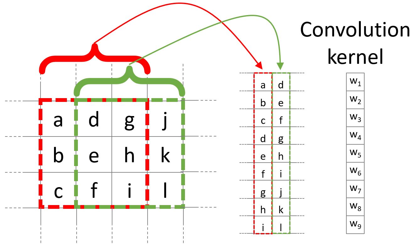
Example of pixel neigborghood arrangements for a \(3 \times 3\) kernel.
In multiple channel case (see equation (1) for \(C\) input channels), all input channels contribute to the output. At the column matrix level, this translates into stacking individual columns from all channels along a single column, and similarly for the kernel weights. Conversely, in order to account for multi-channel output, multiple column matrices are considered, or, equivalently, the column matrix and the corresponding kernel weights have an extra dimension along \(C_{out}\).
In this setting, striding consists in applying the im2col operation on a subset of the input, while dilation consists in building columns according to the dilation factor, using non-immediate neighbors. Last, padding can be achieved by adding zeros (or the padded values of choice) along the columns of the column matrix.
Owing to the opportunity for vectorization and cache friendliness of the general matrix multiply operations (GEMM), the resulting gains in efficiency outweigh the additional memory consumption due to duplication of values in the column image, since every value in the input image will be replicated in as many locations as the neighbors it participates to (see figure 2).
The \(im2col\) operation is easily reversible. This will be considered for deep neural networks training steps where the backward gradient propagation is applied in order to optimize the network parameters.
INDEXED KERNELS
Given the general interpretation of convolution and its implementation as given in the previous sections, the extension of convolution from rectangular lattices to more general arrangements is now straightforward.
Given an input vector of data and a matrix of indices describing every neighborhood relationships among the elements of the input vectors, a column matrix is constructed by picking elements from the input vector according to each neighborhood in the matrix of indices. Analogously to the case of rectangular lattices, neighborhoods from different input channels are concatenated along individual columns, as are kernel weights. At this point, convolution can be computed as a matrix multiplication.
We will now show how the above procedure can be performed in a vectorized fashion by resorting to advanced indexing. Modern multidimensional array frameworks, such as NumPy, TensorFlow and PyTorch, implement advanced indexing, which consists in indexing multidimensional arrays with other multidimensional arrays of integer values. The integer arrays provide the shape of the output and the indices at which the output values must be picked out of the input array.
In our case, we can use the matrix of indices describing neighborhoods in order to index into the input tensor, producing the column matrix in one pass, both on CPU and GPU devices. Since the indexing operation is differentiable with respect to the input (but not with respect to the indices), a deep learning framework equipped with automatic differentiation capabilities (like PyTorch or TensorFlow) can provide the backward pass automatically as needed.
We will now present a PyTorch implementation of such indexed convolution in a hypothetical case.
We consider in the following example an input tensor with shape \(B, C_{in}, W_{in}\), where \(B\) is the batch size equal to 1, \(C_{in}\) is the number of channels equal to 2, or features, and \(W_{in}\) is the width equal to 5, i.e. the number of elements per channel,
input = torch.ones(1, 2, 5)
and a specification of neighbors as an indices tensor with shape \(K, W_{out}\), where \(K\) is the size of the convolution kernel equal to 3 and \(W_{out}\) equal to 4 is the number of elements per channel in the output
indices = torch.tensor([[ 0, 0, 3, 4],
                        [ 1, 2, 4, 0],
                        [ 2, 3, 0, 1]])
where values, arbitrarily chosen in this example, represent the indices of 4 neighborhoods of size 3 (i.e. neighborhoods are laid out along columns). The number of columns corresponds to the number of neighborhoods, i.e. dot products, that will be computed during the matrix multiply, hence they correspond to the size of the output per channel.
The weight tensor describing the convolution kernels has shape \([C_{out}, C_{in}, K]\), where \(C_{out}\) equal to 3 is the number of channels, or features, in the output. The bias is a column vector of size \(C_{out}\).
weight = torch.ones(3, 2, 3)
bias = torch.zeros(3)
At this point we can proceed to use advanced indexing to build the column matrix according to indices.
col = input[..., indices]
Here we are indexing a \(B, C_{in}, W_{in}\) tensor with a \(K, W_{out}\) tensor, but the indexing operation has to preserve batch and input channels dimensions. To this end, we employ the ellipsis notation \(...\), which prescribes indexing to be replicated over all dimensions except the last. This operation produces a tensor shaped \(B, C_{in}, K, W_{out}\), i.e. \(1, 2, 3, 4\).
As noted above, the column matrix needs values from neighborhoods for all input channels concatenated along individual columns. This is achieved by reshaping the col tensor so that \(C_{in}\) and \(K\) dimensions are concatenated:
B = input.shape[0]
W_out = indices.shape[1]

col = col.view(B, -1, W_out)
The columns in the col tensor are now a concatenation of 3 values (the size of the kernel) per input channel, resulting in a \(B, K \cdot C_{in}, W_{out}\). Note that the col tensor is still organized in batches.
At this point, weights must be arranged so that weights from different channels are concatenated along columns as well:
C_out = weight.shape[0]
weight_col = weight.view(C_out, -1)
which leads from a \(C_{out}, C_{in}, K\) to a \(C_{out}, K \cdot C_{in}\) tensor.
Multiplying the weight_col and col matrices will now perform the vectorized dot product corresponding to the convolution:
out = torch.matmul(weight_col, col)
Note that we are multiplying a \(C_{out}, K \cdot C_{in}\) tensor by a \(B, K \cdot C_{in}, W_{out}\) tensor, to obtain a \(B, C_{out}, W_{out}\) tensor. In this case, the \(B\) dimension has been automatically broadcast, without extra allocations.
In case bias is used in the convolution, it must be added to each element of the output, i.e. a constant is summed to all values per output channel. In this case, bias is a tensor of shape \(C_{out}\), so we can perform the operation by again relying on broadcasting on the first \(B\) and last \(W_{out}\) dimension:
out += bias.unsqueeze(1)
Padding can be handled by prescribing a placeholder value, e.g. \(-1\), in the matrix of indices. The following instruction shows an example of such a strategy:
indices = torch.tensor([[-1, 0, 3, 4],
                        [ 1, 2, 4, 0],
                        [ 2, 3, 0, 1]])
The location can be used to set the corresponding input to the zero padded value, though multiplication of the input by a binary mask. Once the mask has been computed, the placeholder can safely be replaced with a valid index so that advanced indexing succeeds.
indices = indices.clone()
padded = indices == -1
indices[padded] = 0

mask = torch.tensor([1.0, 0.0])
mask = mask[..., padded.long()]

col = input[..., indices] * mask
POOLING
Pooling Operation
In deep neural networks, convolutions are often associated with pooling layers. They allow feature maps down-sampling thus reducing the number of network parameters and so the time of the computation. In addition, pooling improves feature detection robustness by achieving spatial invariance [SMullerB10].
The pooling operation can be defined as:
where \(O_i\) is the output pixel \(i\), \(f\) a function, \(I_{N_i}\) the neighborhood of the input pixel \(i\) of a given input feature map \(I\). The pooling function \(f\) provided on equation (2) is applied on \(I_{N_i}\) using a sliding window. \(f\) can be of various forms, for example an average, a Softmax, a convolution or a max. The use of a stride greater than 2 on the sliding window translation enables to sub-sample the data. With convolutional networks, a max-pooling layer with stride 2 and width 3 is typically considered moving to a 2 times coarser feature maps scale after having applied some standard convolution layers. This proved to reduce network overfit while improving task accuracy [KSH12].
Indexed Pooling
Following the same procedure as for convolution described in section 3, we can use the matrix of indices to produce the column matrix of the input and apply, in one pass, the pooling function to each column.
For instance, a PyTorch implementation of the indexed pooling, in the same hypothetical case as presented in section 3, with max as the pooling function is:
col = input[..., indices]
out = torch.max(col, 2)
APPLICATION EXAMPLE: THE HEXAGONAL CASE
The indexed convolution and pooling can be applied to any pixel organization, as soon as one provides the list of the neighbors of each pixel. Although the method is generic, we first developed it to be able to apply Deep Learning technic to the hexagonal grid images of the Cherenkov Telescope Array (from NectarCam, citealt{2013arXiv1307.4545G}; LSTCam, citealt{ambrosi2013cherenkov}; and FlashCam, citealt{2012AIPC.1505..777P}). Even if hexagonal data processing is not usual for general public applications, several other specific sensors make use of hexagonal sampling. The Lytro light field camera [CLKT13] is a consumer electronic device example. Several Physics experiments also make use of hexagonal grid sensors, such as the H.E.S.S. camera [BCG+14] or the XENON1T detector [Scovell13]. Hexagonal lattice is also used for medical sensors, such as DEPFET [NBB+00] or retina implant system [SHH+99].
Moreover, hexagonal lattice is a well-known and studied grid [AHA12, HPCW18, SMOK02, SSO10] and offers advantages compared to square lattice [MSC01] such as higher sampling density and a better representation of curves. In addition, some more benefits have been shown by [AHA12, HJ05, Sou14] such as equidistant neighborhood, clearly defined connectivity, smaller quantization error.
However, processing hexagonal lattice images with standard deep learning frameworks requires specific data manipulation and computations that need to be optimized on CPUs as well as GPUs. This section proposes a method to efficiently handle hexagonal data without any preprocessing as a demonstration of the use of indexed convolutions. We first describe how to build the index matrix for hexagonal lattice images needed by the indexed convolution.
For easy comparison, we want to validate our methods on datasets with well-known use cases (e.g. a classification task) and performances. To our knowledge, there is no reference hexagonal image dataset for deep learning. So, following HexaConv paper [HPCW18] we constructed two datasets with hexagonal images based on well-established square pixel image datasets dedicated to classification tasks: CIFAR-10 and AID. This enables our method to be compared with classical square pixels processing in a standardized way.
Indexing the hexagonal lattice and the neighbors’ matrix
As described in section 3, in addition to the image itself, one needs to feed the indexed convolution (or pooling) with the list of the considered neighbors for each pixel of interest, the matrix of indices. In the case of images with a hexagonal grid, provided a given pixel addressing system, a simple method to retrieve these neighbors is proposed.
Several addressing systems exist to handle images with such lattice, among others: offset [Sou14], ASA [Rum10], HIP [MSC01], axial - also named orthogonal or 2-axis obliques [AHA12, Sou14]. The latter is complete, unique, convertible to and from Cartesian lattice and efficient [HJ05]. It offers a straightforward conversion from hexagonal to Cartesian grid, stretching the converted image, as shown in figure 3, but preserving the true neighborhood of the pixels.
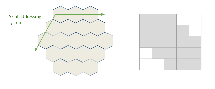
Hexagonal to Cartesian grid conversion with the axial addressing system.
Our method relies on the axial addressing system to build an index matrix of hexagonal grid images. Assuming that a hexagonal image is stored as a vector and that we have the indices of the pixels of the vector images represented in the hexagonal grid, one can convert it to an index matrix thanks to the axial addressing system. Then, building the list of neighbors, the matrix of indices, consists in applying the desired kernel represented in the axial addressing system to the index matrix for each pixel of interest.
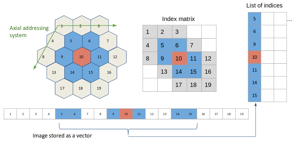
Building the matrix of indices for an image with a hexagonal grid. The image is stored as a vector, and the indices of the vector are represented in the hexagonal lattice. Thanks to the axial addressing system, this representation is converted to a rectangular matrix, the index matrix. The neighbors of each pixel of interest (in red) are retrieved by applying the desired kernel (here the nearest neighbors in the hexagonal lattice, in blue) to the index matrix.
An example is proposed on figure 4 <fig_hexagonal_kernel>, with the kernel of the nearest neighbors in the hexagonal lattice. Regarding the implementation, one has to define in advance the kernel to use as a mask to be applied to the index matrix, for the latter example:
kernel = [[1, 1, 0],
          [1, 1, 1],
          [0, 1, 1]]
Experiment on CIFAR-10
The indexed convolution method, in the special case of hexagonal grid images, has been validated on the CIFAR-10 dataset. For this experiment and the one on the AID dataset (see Sec. 5.3), we compare our results with the two baseline networks of HexaConv paper [HPCW18]. These networks do not include group convolutions and are trained respectively on square and hexagonal grid image versions of CIFAR-10. The network trained on the hexagonal grid CIFAR-10 consists of masked convolutions. To allow a fair comparison, we use the same experimental conditions, except for the Deep Learning framework and the square to hexagonal grid image transformation of the datasets.
The CIFAR-10 dataset is composed of 60000 tiny color images of size 32x32 with square pixels. Each image is associated with the class of its foreground object. This is one of the reference databases for image classification tasks in the machine learning community. By converting this square pixel database into its hexagonal pixel counterpart, this enables to compare hexagonal and square pixel processing in different case studies for image classification. This way, the same network with:
standard convolutions (square kernels),
indexed convolutions (square kernels),
indexed convolutions (hexagonal kernels),
has been trained and tested, respectively on the dataset for the square kernels and its hexagonal version for the hexagonal kernels. For reproducibility, the experiment has been repeated 10 times with different weights initialization, but using the same random seeds (i.e. same weights initialization values) for all three implementations of the network.
Building a Hexagonal CIFAR-10 Dataset
The first step is to transform the dataset in a hexagonal one. Compared to a rectangular grid, an hexagonal grid has one line out of two shifted of half a pixel (see figure 5 <fig_square_to_hexa>). Square pixels (orange grid) cannot be rearranged directly in a hexagonal grid (blue grid). For these shifted lines, pixels have to be interpolated from the integer position pixels of the rectangular grid. The interpolation chosen here is the average of the two consecutive horizontal pixels. A fancier method could have been to take into account all the six square pixels contributing to the hexagonal one, in proportion to their involved surface. In that case, the both pixels retained for our interpolation method would cover 90.4% of the surface of the interpolated hexagonal pixel.
Figure 6 shows a conversion example, one can observe that the interpolation method is rough as one can see on the back legs of the horse so that hexagonal processing experiments suffer from some input image distortion. However, our preliminary experiments did not show strong classification accuracy difference between such conversion and a higher quality one.
Then the images are stored as vectors and the index matrix based on the axial addressing system is built. Before feeding the network, the images are standardized and whitened using a PCA, following citealt{hoogeboom2018hexaconv}.
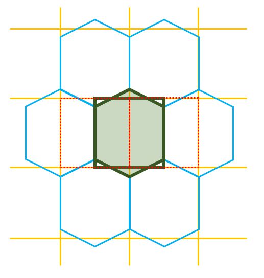
Resampling of rectangular grid (orange) images to hexagonal grid one (blue). One line of two in the hexagonal lattice is shifted by half a pixel compared to the corresponding line in the square lattice. The interpolated hexagonal pixel (with a green background) is the average of the two corresponding square pixels (with red dashed borders).
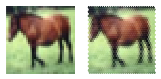
Example of an image from CIFAR-10 dataset resampled to hexagonal grid.
Network model
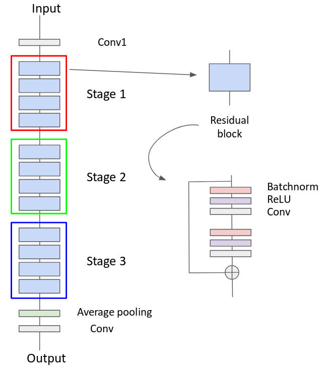
ResNet model used for the experiment on CIFAR-10.
conv1 |
stage 1 |
stage 2 |
stage 3 |
|
|---|---|---|---|---|
Hexagonal kernels |
17 |
17 |
35 |
69 |
Square kernels |
15 |
15 |
31 |
61 |
The network used for this experiment is described in section 5.1 of [HPCW18] and relies on a ResNet architecture [HZRS15]. As shown in figure 7, it consists of a convolution, 3 stages with 4 residual blocks each, a pooling layer and a final convolution. The down-sampling between two stages is achieved by a convolution of kernel size 1x1 and stride 2. After the last stage, feature maps are squeezed to a single pixel (1x1 feature maps) by the use of an average pooling over the whole feature maps. Then a final 1x1 convolution (equivalent to a fully connected layer) is applied to obtain the class scores. Three networks have been implemented in PyTorch, one with built-in convolutions (square kernels) and two with indexed convolutions (one with square kernels and one with hexagonal kernels). Rectangular grid image versions have convolution kernels of size 3x3 (9 pixels) while the one for hexagonal grid images has hexagonal convolution kernels of the nearest neighbors (7 pixels). The number of features per layer is set differently, as shown in table [tab:cifar-features], depending on the network so that the total number of parameters of all three networks are close, ensuring the comparison to be fair. These networks have been trained with the stochastic gradient descent as optimizer with a momentum of 0.9, a weight decay of 0.001 and with a learning rate of 0.05 decayed by 0.1 at epoch 50, 100 and 150 for a total of 300 epochs.
Results
As shown in table [tab:cifar-results], all three networks with hexagonal indexed convolutions, square indexed convolutions and square standard convolutions exhibit similar performances on the CIFAR-10 dataset. The difference between the hexagonal kernel and the square kernel with standard convolution on the one hand and between both square kernel is not significant, according to the Student T test. For the same number of parameters, the hexagonal kernel model gives slightly better accuracy than the square kernel one in the context of indexed convolution, even if the images have been roughly interpolated for hexagonal image processing. However, to satisfy this equivalence in the number of parameters, since hexagonal convolutions involve fewer neighbors than the squared counterpart, some more neurons are added all along the network architecture. This leads to a larger number of data representations that are combined to achieve the task. One can then say that Hexagonal convolution provides richer features for the same price in the parameters count. This may also compensate for the image distortions introduced when converting input images to hexagonal sampling. Such distortions actually sat Hexagonal processing in an unfavourable initial state but the hexagonal processing compensated and slightly outperformed the standard approach.
citet{hoogeboom2018hexaconv} carried out a similar experiment and observed the same accuracy difference between hexagonal and square convolutions processing despite a shift in the absolute accuracy values (88.75 for hexagonal images, 88.5 for square ones) that can be explained by different image interpolation methods, different weights initialization and the use of different frameworks.
Hexagonal kernels (i.c.) |
Square kernels (i.c.) |
Square kernels |
|---|---|---|
\(88.51 \pm 0.21\) |
\(88.27 \pm 0.23\) |
\(88.39 \pm 0.48\) |
Experiment on AID
Similar to the experiment on CIFAR-10, the indexed convolution has been validated on Aerial Images Dataset (AID) [XHH+16]. The AID dataset consists of 10000 RGB images of size 600x600 within 30 classes of aerial scene type. Similar to section 5.2, the same network with standard convolutions (square kernels) and then with indexed convolutions (square kernels and hexagonal kernels) have been trained and tested, respectively on the dataset for the square kernels and its hexagonal version for the hexagonal kernels. The experiment has also been repeated ten times, but with the same network initialization and different random split between training set and validating set, following citet{hoogeboom2018hexaconv}.
Building a Hexagonal AID Dataset
After resizing the images to 64x64 pixels, the dataset is transformed to a hexagonal one, as shown figure 8, in the same way as in section 5.2.1. Then the images are standardized.
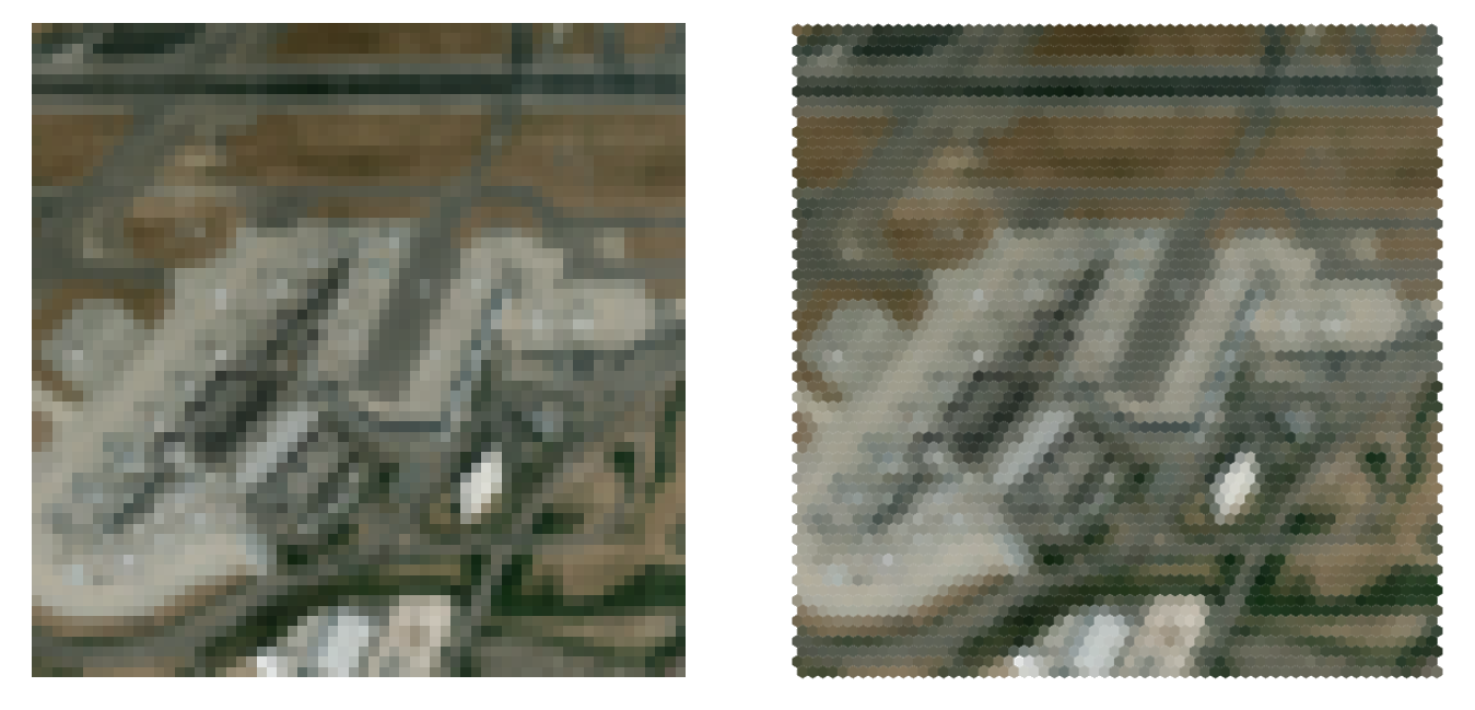
Example of an image from AID dataset resized to 64x64 pixels and resampled to hexagonal grid.
Network
conv1 |
stage 1 |
stage 2 |
stage 3 |
|
|---|---|---|---|---|
Hexagonal kernels |
42 |
42 |
83 |
166 |
Square kernels |
37 |
37 |
74 |
146 |
The network considered in this experiment is still a ResNet architecture but adapted to this specific dataset. One follows the setup proposed in section 5.2 of citealt{hoogeboom2018hexaconv}. Three networks have been implemented and trained in the same way described in section 5.2.2, with the number of features per layer described in table [tab:aid-features].
Results
As shown in table [tab:aid-results], all three networks with hexagonal convolutions and square convolutions do not exhibit a significant difference in performances on the AID dataset. Again, no accuracy loss is observed in the hexagonal processing case study despite the rough image re-sampling.
However, unlike on the CIFAR-10 experiment, we don’t observe a better accuracy of the model with hexagonal kernels, as emphasized in [HPCW18].
Hexagonal kernels (i.c.) |
Square kernels (i.c.) |
Square kernels |
|---|---|---|
\(79.81 \pm 0.73\) |
\(79.88 \pm 0.82\) |
\(79.85 \pm 0.50\) |
ACKNOWLEDGEMENTS
BIBLIOGRAPHY
Giovanni Ambrosi, Y Awane, H Baba, and others. The cherenkov telescope array large size telescope. arXiv preprint arXiv:1307.4565, 2013.
J. Bolmont, P. Corona, P. Gauron, and others. The camera of the fifth h.e.s.s. telescope. part i: system description. Nuclear Instruments and Methods in Physics Research Section A: Accelerators, Spectrometers, Detectors and Associated Equipment, 761:46 – 57, 2014. URL: http://www.sciencedirect.com/science/article/pii/S0168900214006469, doi:https://doi.org/10.1016/j.nima.2014.05.093.
Donghyeon Cho, Minhaeng Lee, Sunyeong Kim, and Yu-Wing Tai. Modeling the calibration pipeline of the lytro camera for high quality light-field image reconstruction. In Proceedings of the IEEE International Conference on Computer Vision, 3280–3287. 2013.
Kaiming He, Xiangyu Zhang, Shaoqing Ren, and Jian Sun. Deep residual learning for image recognition. CoRR, 2015. URL: http://arxiv.org/abs/1512.03385, arXiv:1512.03385.
Xiangjian He and Wenjing Jia. Hexagonal structure for intelligent vision. In Information and Communication Technologies, 2005. ICICT 2005. First International Conference on, 52–64. IEEE, 2005.
Tim Lukas Holch, Idan Shilon, Matthias Büchele, and others. Probing convolutional neural networks for event reconstruction in $gamma$-ray astronomy with cherenkov telescopes. arXiv preprint arXiv:1711.06298, 2017.
M. Holschneider, R. Kronland-Martinet, J. Morlet, and Ph. Tchamitchian. A real-time algorithm for signal analysis with the help of the wavelet transform. In Jean-Michel Combes, Alexander Grossmann, and Philippe Tchamitchian, editors, Wavelets, 286–297. Berlin, Heidelberg, 1990. Springer Berlin Heidelberg.
Emiel Hoogeboom, Jorn W.T. Peters, Taco S. Cohen, and Max Welling. Hexaconv. In International Conference on Learning Representations. 2018.
Ulrich Katz. A neutrino telescope deep in the Mediterranean Sea. CERN Cour., 52N6:31–33, 2012.
Alex Krizhevsky, Ilya Sutskever, and Geoffrey E Hinton. Imagenet classification with deep convolutional neural networks. In Advances in neural information processing systems, 1097–1105. 2012.
L Middleton, J Sivaswamy, and G Coghill. The fft in a hexagonalimage processing framework. New Zealand Conference on Image and Vision Computing (IVCNZ 2001), pages 231–236, 2001.
Wolfgang Neeser, M Bocker, Peter Buchholz, and others. The depfet pixel bioscope. IEEE Transactions on Nuclear Science, 47(3):1246–1250, 2000.
Nicholas I Rummelt. Array set addressing: enabling efficient hexagonally sampled image processing. University of Florida, 2010.
Hidenori Sato, Hiroto Matsuoka, Akira Onozawa, and Hitoshi Kitazawa. Hexagonal image representation for 3-d photorealistic reconstruction. In Pattern Recognition, 2002. Proceedings. 16th International Conference on, volume 2, 672–676. IEEE, 2002.
Dominik Scherer, Andreas Müller, and Sven Behnke. Evaluation of pooling operations in convolutional architectures for object recognition. In Artificial Neural Networks–ICANN 2010, pages 92–101. Springer, 2010.
Markus Schwarz, Ralf Hauschild, Bedrich J Hosticka, and others. Single-chip cmos image sensors for a retina implant system. IEEE Transactions on Circuits and Systems II: Analog and Digital Signal Processing, 46(7):870–877, 1999.
Tetsuo Shima, Shigeki Sugimoto, and Masatoshi Okutomi. Comparison of image alignment on hexagonal and square lattices. In Image Processing (ICIP), 2010 17th IEEE International Conference on, 141–144. IEEE, 2010.
Robert van de Geijn and Kazushige Goto. BLAS (Basic Linear Algebra Subprograms), pages 157–164. Springer US, Boston, MA, 2011. URL: https://doi.org/10.1007/978-0-387-09766-4_84, doi:10.1007/978-0-387-09766-4_84.
Gui-Song Xia, Jingwen Hu, Fan Hu, and others. AID: A benchmark dataset for performance evaluation of aerial scene classification. CoRR, 2016. URL: http://arxiv.org/abs/1608.05167, arXiv:1608.05167.
J. Glicenstein, M. Barcelo, J. Barrio, and others. The NectarCAM camera project. ArXiv e-prints, July 2013. arXiv:1307.4545.
G. Pühlhofer, C. Bauer, A. Biland, and others. FlashCam: A fully digital camera for CTA telescopes. In F. A. Aharonian, W. Hofmann, and F. M. Rieger, editors, American Institute of Physics Conference Series, volume 1505 of American Institute of Physics Conference Series, 777–780. December 2012. arXiv:1211.3684, doi:10.1063/1.4772375.
COMMENTS/DISCUSSION
This paper introduces indexed convolution and pooling operators for images presenting pixels arranged in non-Cartesian lattices. These operators have been validated on standard images as well as on the special case of hexagonal lattice images, exhibiting similar performances as standard convolutions and therefore showing that the indexed convolution works as expected. However, the indexed method is much more general and can be applied to any grid of data, enabling unconventional image representation to be addressed without any pre-processing. This differs from other approaches such as image re-sampling combined with masked convolutions [HPCW18] or oversampling to square lattice [HSBuchele+17] that actually require additional pre-processing. Moreover, both methods increase the size of the transformed image (adding useless pixels of padding value for the resampled image to be rectangular and / or multiplying the number of existing pixels) and are restricted to regular grids. On the other hand, they make use of out the box operators already available in current deep learning frameworks.
The approach proposed in this paper is not limited to hexagonal lattice and only needs the index matrices to be built prior the training and inference processes, one for each convolution of different input size. No additional pre-processing of the image is then required to apply convolution and pooling kernels. However, the current implementation in Python shows a decrease in computing performances compared to the convolution method implemented in Pytorch. We have observed an increase of RAM usage of factors varying between 1 and 3 and training times of factors varying between 4 and 8 on GPU (depending on the GPU model), of factor 1.5 on CPU (but slightly faster than masked convolutions on CPU) depending on the network used.
These drawbacks are actually related to the use of un-optimized codes and work is carried out to fix this by the use of optimized CUDA and C++ implementations.
As a future work, we will use the indexed operations for the analysis of hexagonal grid images of CTA. We also plan to experiment with arbitrary kernels, which are another benefit of the indexed operations, for the convolution (e.g. retina like kernel with more density in the center, see the example in the github repository).